

In this tutorial, we will explore a basic workflow to train and evaluate a model to classify text. Note that there are many important aspects not covered in what follows, such as exploratory data analysis (EDA) or hyper-parameter optimisation.
In this tutorial, we will take a real example of the 20 newsgroups dataset, popular among the NLP community. In this dataset, each sample is labelled as one of 20 categories, such as religion or space.
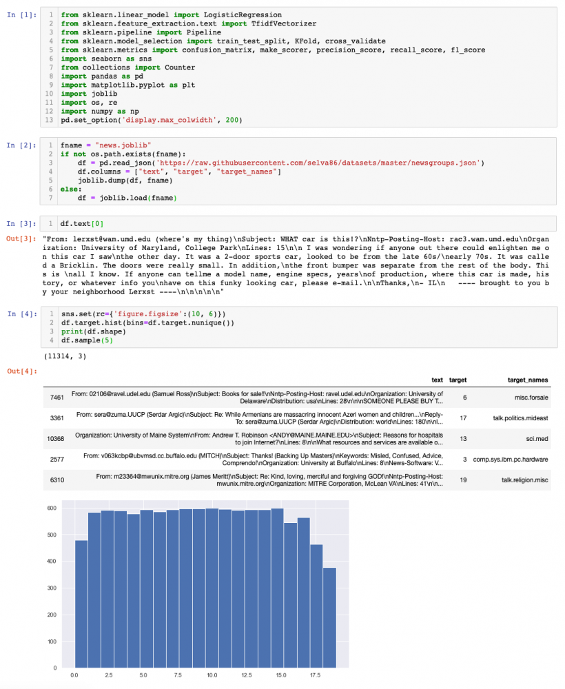
We can see that this is a balanced dataset, as all classes are represented more or less equally. The following cell just finds the mapping from target name to target-ID, which will be useful later.

List of Contents
The tutorial is organised as follows:
- Data Cleaning: some easy steps to remove parts of and / or standardise the data.
- Data Representation: before being able to train a model, we need to represent data (in our case text) in some numerical shape, both inputs and labels. In our case, labels are already encoded. For inputs, this step usually reduces to feature extraction.
- Binary classification: we will first address the classification problem by simplifying it to a binary classification, i.e. labels 0…9 vs 10…19, which happens to be more or less balanced problem. This will be carried out by using Logistic Regression. In addition to be an easy to start algorithm, this will be useful to review how to measure the performance for a trained model.
- Multi-class Classification: we will extend the previous approach for our scenario with 20 classes using two different methodologies, and obtain performance results for the given dataset.
- Further work: a proposal of tentative tasks to continue learning
1. Data Cleaning
An important first step in any ML project is to clean data. In this case, all texts start with a preamble, see the samples in cell 3. Also, we will perform other simple operations. Note that a very important step before (and after) cleaning data is EDA (here omitted), so that you might detect data patterns and issues.
2. Data Representation
In every ML-based system, there is a block dedicated to data representation. That is, a translation from raw input (in our case the text for the section and the associated class) to some representation the model can learn from. One of the key steps involved in data representation is feature extraction, next explained.
TF-IDF feature extraction
For this tutorial, we will just use TF-IDF, see this for reference. In layman terms, TF-IDF represents each piece of text as a long vector, whose components are associated to a different word each (or groups of words if ngrams are considered), and its value is related to how important that word is to characterise the document. Again, for a more comprehensive definition, see reference or the literature.
![]()
3. Binary Classification
We will start using Logistic Regression (LR), a linear model that in its simplest form allows to separate two classes, i.e. perform binary classification. The basis of LR is to apply the sigmoid function to the result of a linear regression. As the sigmoid outputs always a value between 0 and 1, one can interpret the result as the probability for one of the classes. Then, mathematically we have:
![]()
with
![]()
where x represents the input features, and W the learned weights representing the model. For a more extensive description of LR, please see e.g. this reference
Let’s binarise the labels so that classes 0–9 will be in one bucket, and 10–19 in another one. This scenario is still balanced.
We will measure the performance of our model using precision, recall, and f1-score. They are defined as follows:
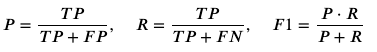
where TP, FP, FN refer to the true positives, false positives, and false negatives, respectively. See more info here. These metrics refer to a binary classification. Imagine we are detecting spam, and that's considered to be the "positive" class. Then, precision is the probability of being true spam when model has classified it as spam, whereas recall is the other way around: probability of classifying as spam, when the sample is true spam. The F-score can be considered as an aggregation of both metrics into a single number. I will defer the interested reader to the aforementioned article. For experienced readers, it is also interesting this more advanced and relatively recent paper.
Note that we will define the scorers with average=Macro. This is more important for the multi-class than the binary case, but basically it means that for each class we consider all other classes to be the negative class, and compute the given metric. Once we have the scorer for each class, they are averaged. For a balanced scenario as the one here, this is reasonable. Read more about this e.g. here.

We will perform cross-validation (CV) to measure the performance of our model. CV is a method to obtain an unbiased estimation of a model's performance. It is especially suited for small datasets, see more details here.
In particular, we will apply K-fold CV, with K=3. As a sanity check, I usually prefer to do shuffle=True as otherwise sklearn KFold would split as {1...N}, {N + 1...2N} etc, which might lead to problems if data has some order.
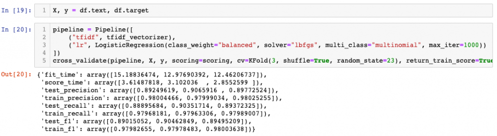
We will evaluate the model with only unigrams, or using unigrams+bigrams. In this regard, notice how useful the CV framework offered by sklearn together with the pipeline class are. These allow you to define the different steps of your ML system, and just by modifying the pipeline, you can run again testing for a different configuration and compare. I recommend taking a look at pipelines in combination with GridSearchCV, see e.g. this.
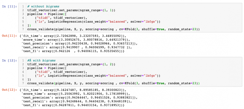
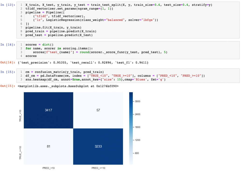
We can see how bigrams improve a bit the predictive power, at the cost of fit and score time. Feel free to try with higher-order ngrams, but you will see that at some point adding more features induces overfitting. Plus, it looks like all folds are similar, so from here I will just do train-test and check the confusion matrix, which simply puts together TP, TN, FP, FN in a matrix.
Showing the confusion matrix as percentages (normalised by the true labels):
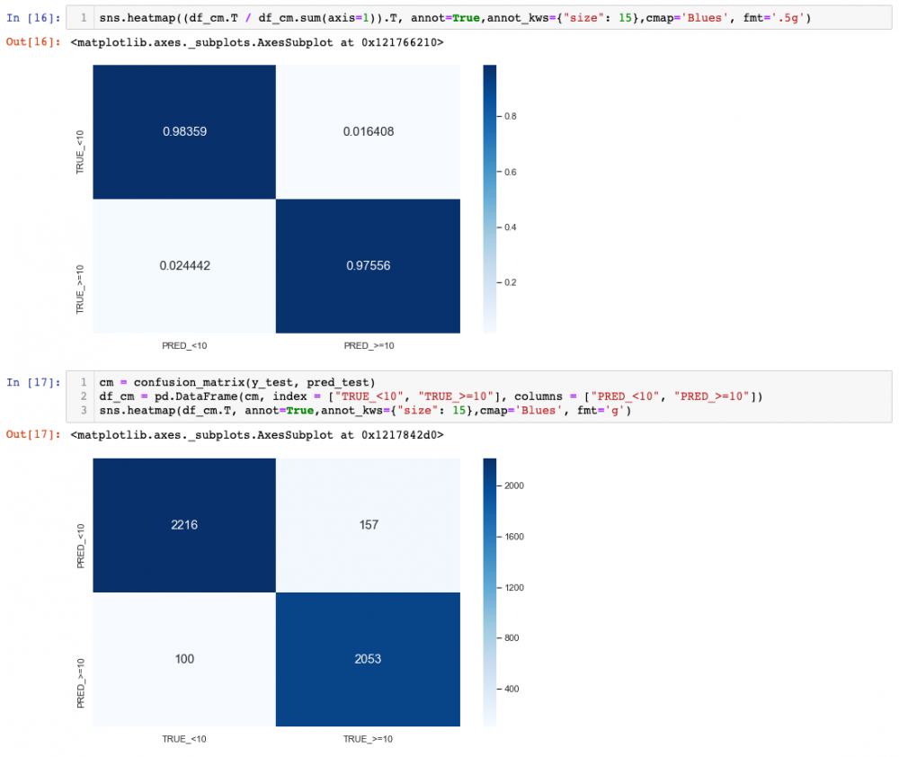
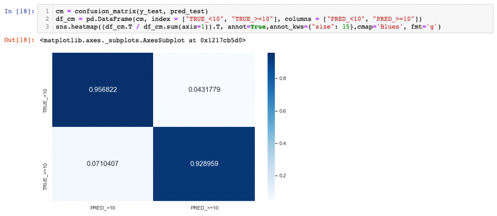
We can see how the results are a bit worse for test (obviously!), but still pretty decent. As a curiosity, notice that the way we normalised, the bottom-right corner is actually recall
4. Multi-class Classification
Let’s deal now with the real 20 classes problem. For this, we are going to use an extension of Logistic Regression called Multinomial Logistic Regression. Don’t be scared by the name, it is quite simple. Again, I’m going to refer to Wikipedia for the meat, but just to get some intuition, the idea is to have a set of weights W(k) for each class k and then consider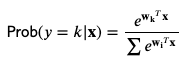
so we keep the class whose associated probability is higher.
In addition to the multinomial extension, one can deal with the multi-class case performing a one-vs-all strategy. This means that for each class, we compute a model where that class is the positive class, and the rest belong to the negative class. At prediction time, we select the class whose model predicts the higuest score. See this for more details.
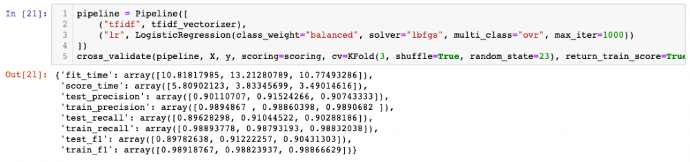
So faster and better results with one-vs-all, at least with current hyper-parameters. Besides, notice that, again, all folds behave similarly. Just for a quick check, let's see how the confusion matrix looks like when we have 20 classes (using the pipeline with one-vs-all)
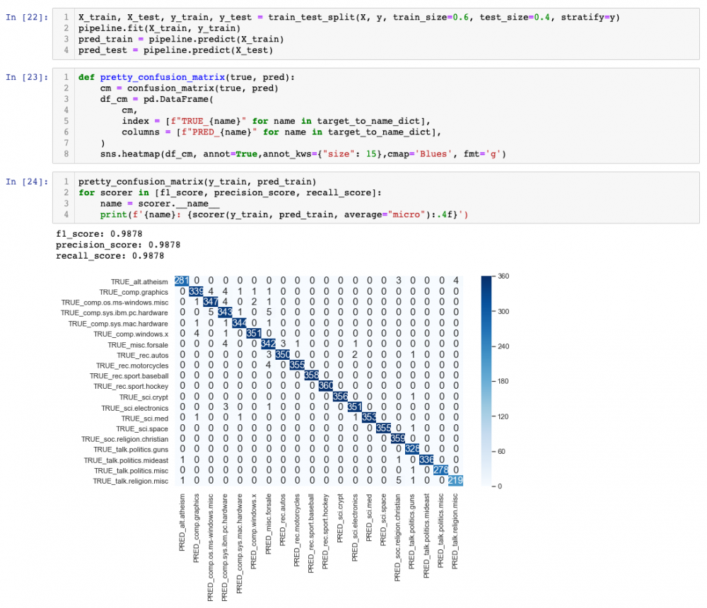
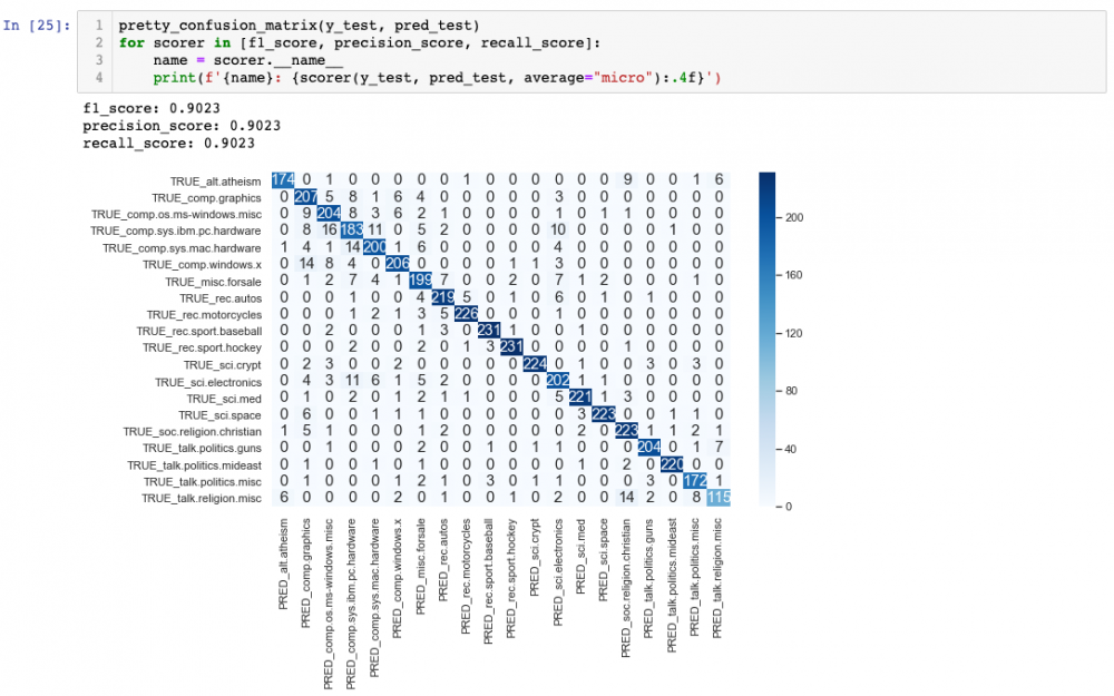
We can see some interesting confusions here. For example,hardware_PC, hardware_mac-electronics or religion-guns. Also, we can see a bit of overfitting, given that the performance on the training set is way higher than on the test set. This is something that could potentially be improved with hyperparameter tuning, especially increasing regularisation.
Further work
And with this we got to the end of this tutorial. Some more ideas or directions to explore after reading this are:
- Hyper-parameter optimisation: use e.g. GridSearchCV from sklearn. For more advanced readers, consider Bayesian optimisation, e.g. with hyperopt.
- Better model evaluation: learning curves, overfitting vs underfitting analysis, etc
- More feature extraction: add more features apart from / in addition to TF-IDF. For example:
- Count entities like names, locations, etc, and use them as extra features. This can potentially use a Named Entity Recognition (NER) system. I recommend you to take a look at spaCy.
- Topic features: extract topics to learn more about the dataset / add them as features to improve the classifier. I recommend here using LDA with the gensim library.
- Use word embeddings based features.
- Use other classical ML algorithms, usually good in overfitting scenarios, e.g. SVM, Random Forest
- Deep Learning based model, and also transfer learning. I recommend here using FastAI and the ULMFit methodology.
More Tutorials to Practice your Skills on:
- Introduction to Missing Data Imputation
- Introduction to Pandas
- Hyperparameter tuning in XGBoost
- Introduction to CoordConv Architecture: Deep Learning
- Unit testing with PySpark
- Getting started with XGBoost

By Marc Torrellas Socastro.
Marc received a PhD with honors (2011-2015) in Wireless Communications and Information Theory from Universitat Politècnica de Catalunya (UPC), where he obtained his MSc. in Telecommunications (2006-2011), and his MSc. Information Technologies (Merit Master, 2011-2013). Since 2015, he has worked as a Data Scientist for Zhilabs in Barcelona, providing in-depth data analytics to telco providers; Darktrace in Cambridge, UK, providing ML-based cybersecurity services; Eigen Technologies in London, providing ML and NLP based products and services, focused on extracting unstructured information from legal and financial documents; and Streetbees in London, providing market research and insights into communities by leveraging ML and NLP concepts.
-1.png)
Enquire now
Fill out the following form and we’ll contact you within one business day to discuss and answer any questions you have about the programme. We look forward to speaking with you.
