

Introduction
The recent advances of machine learning and growing amounts of available data have had a great impact on the field of Natural Language Processing (NLP). They facilitated development of new neural architectures and led to strong improvements on many NLP tasks, such as machine translation or text classification. One advancement of particular importance is the development of models which build good quality, machine-readable representations of word meanings. These representations, often referred to as word embeddings, are vectors which can be used as features in neural models that process text data.
The main aim of this tutorial is to provide (1) an intuitive explanation of Skip-gram — a well-known model for creating word embeddings and (2) a guide for training your own embeddings and using them as input in a simple neural model. In particular, you will learn how to use the implementation of Skip-gram provided by the gensim library and use keras to implement a model for the part-of-speech tagging task which will make use of your embeddings.
This tutorial assumes that the reader is familiar with Python and has some experience with developing simple neural architectures. Before you begin make sure you have installed the following libraries: nltk, genism, tensorflow and numpy.
A bit of background
In contrast to traditional NLP approaches which associate words with discrete representations, vector space models of meaning embed each word into a continuous vector space in which words can be easily compared for similarity. They are based on the distributional hypothesis stating that a word’s meaning can be inferred from the contexts it appears in. Following this hypothesis, words are represented by means of their neighbours — each word is associated with a vector that encodes information about its co-occurrence with other words in the vocabulary. For example, lemon would be defined in terms of words such as juice, zest, curd or squeeze, providing an indication that it is a type of fruit. Representations built in such a way demonstrate a useful property: vectors of words related in meaning are similar — they lie close to one another in the learned vector space. One common way of measuring this similarity is to use the cosine of the angle between the vectors.
The exact method of constructing word embeddings differs across the models, but most approaches can be categorised as either count-based or predict-based, with the latter utilising neural models. In this tutorial we will focus on one of the most popular neural word-embedding models — Skip-gram. But it is worth noting that there exist many well-performing alternatives like Glove or, more recently proposed, ELMo which builds embeddings using language models. There also exist many extentions to Skip-gram that are widely used and worth looking into, such as Fast-text which exploits the subword information.
Skip-gram
(1) Softmax Objective
Skip-gram’s objective is to predict the contexts of a given target-word. The contexts are immediate neighbours of the target and are retrieved using a window of an arbitrary size n — by capturing n words to the left of the target and n words to its right. For instance, if n=3 in the following example Skip-gram would be trained to predict all words highlighted in yellow for the word prickles:
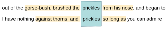
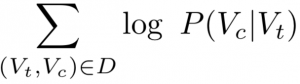
During training the model is exposed to data pairs (Vt, Vc), where V is the vocabulary and t, c are indexes of a target-word and one of its context-words. For the above example the training data would contain pairs like (prickles, nose) and (prickles, thorns). The original Skip-gram’s objective is to maximise P(Vc|Vt) — the probability of Vc being predicted as Vt’s context for all training pairs. If we define the set of all training pairs as D we can formulate this objective as maximising the following expression:
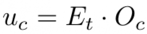
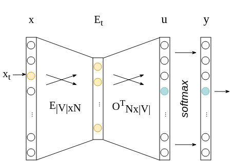
To calculate P(Vc|Vt) we will need a means to quantify the closeness of the target-word Vt and the context-word Vc. In Skip-gram this closeness is computed using the dot product between the input-embedding of the target and the output-embedding of the context. The difference between input-embeddings and output-embeddings lies in that the former represent words when they serve as a target, while the latter when they act as another word’s contexts. Once the model is trained it is usually the input-embedding matrix that is taken as the final word embeddings and used in downstream tasks. It is important to realise this distinction and the fact that in Skip-gram each word is associated with two separate representations. Now, if we define uc to be the measure of words’ closeness, E to be the matrix holding input-embeddings and O to be the output-embedding matrix we get:
which we can use to compute P(Vc|Vt) using the softmax function:

(2) Architecture
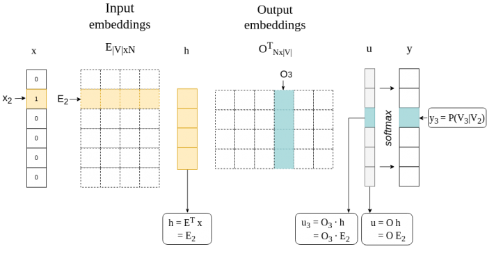
In terms of the architecture, Skip-gram is a simple neural network with only one hidden layer. The input to the network is a one-hot encoded vector representation of a target-word — all of its dimensions are set to zero, apart from the dimension corresponding to the target-word. The output is the probability distribution over all words in the vocabulary which defines the likelihood of a word being selected as the input word’s context:
(3) Negative-Sampling
But there is an issue with the original softmax objective of Skip-gram — it is highly computationally expensive, as it requires scanning through the output-embeddings of all words in the vocabulary in order to calculate the sum from the denominator. And typically such vocabularies contain hundreds of thousands of words. Because of this inefficiency most implementations use an alternative, negative-sampling objective, which rephrases the problem as a set of independent binary classification tasks.
Instead of defining the complete probability distribution over words, the model learns to differentiate between the correct training pairs retrieved from the corpus and the incorrect, randomly generated pairs. For each correct pair the model draws m negative ones — with m being a hyperparameter. All negative samples have the same Vt as the original training pair, but their Vc is drawn from an arbitrary noise distribution. Building on the previous example, for the training pair (prickles, nose) the incorrect ones could be (prickles, worked) or (prickles, truck). The new objective of the model is to maximise the probability of the correct samples coming from the corpus and minimise the corpus probability for the negative samples, such as (prickles, truck).
Let’s set D to be the set of all correct pairs and D’ to denote a set of all negatively sampled |D| × m pairs. We will also define P(C = 1|Vt, Vc) to be the probability of (Vt , Vc) being a correct pair, originating from the corpus. Given this setting, the negative-sampling objective is defined as maximising:

Since this time for each sample we are making a binary decision we define P(C = 1|Vt, Vc) using the sigmoid function:
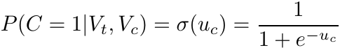
where, as before, uc = Et · Oc. Now, if we plug this into the previous negative-sampling equation and simplify a little we get the following objective:
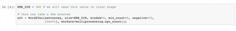
Building our own embeddings
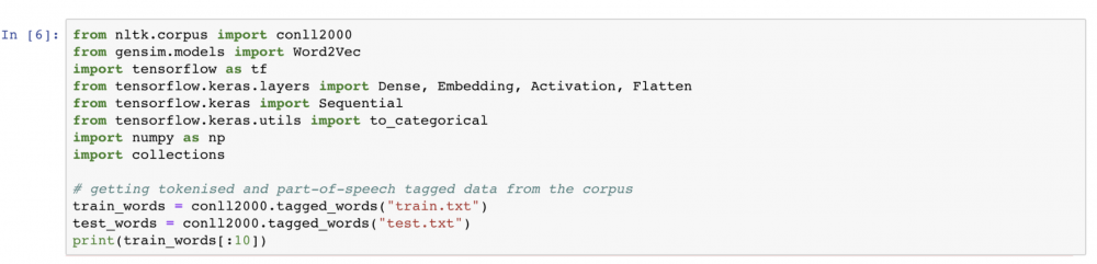
To train our embeddings we will make use of the Skip-gram’s implementation from the Word2Vec module of the gensim library. It provides the algorithms for both Skip-gram and a closely related model — Continuous Bag-of-Words (CBOW). Gensim’s Word2Vec models are trained on a list (or some other iterable) of sentences that have been pre-processed and tokenised — split into separate words and punctuation. Luckily, the NLTK library provides a number of tokenised corpora, such as the Brown corpus, so we can skip the text processing step and jump straight into defining our model!
Before we begin we have to download the necessary NLTK resources using the NLTK data downloader. You can launch it by running the following lines in the Python interpreter. Go to the Corpora tab and double click on ‘brown’ and then on ‘conll2000’ to download the resources (we will need conll2000 later in this tutorial).
For our next steps we will require the following imports:

Let’s start with printing out a few sentences from the Brown corpus to gain some insight into our data.

[['The', 'Fulton', 'County', 'Grand', 'Jury', 'said', 'Friday', 'an', 'investigation', 'of', "Atlanta's", 'recent', 'primary', 'election', 'produced', '``', 'no', 'evidence', "''", 'that', 'any', 'irregularities', 'took', 'place', '.'], ['The', 'jury', 'further', 'said', 'in', 'term-end', 'presentments', 'that', 'the', 'City', 'Executive', 'Committee', ',', 'which', 'had', 'over-all', 'charge', 'of', 'the', 'election', ',', '``', 'deserves', 'the', 'praise', 'and', 'thanks', 'of', 'the', 'City', 'of', 'Atlanta', "''", 'for', 'the', 'manner', 'in', 'which', 'the', 'election', 'was', 'conducted', '.'], ['The', 'September-October', 'term', 'jury', 'had', 'been', 'charged', 'by', 'Fulton', 'Superior', 'Court', 'Judge', 'Durwood', 'Pye', 'to', 'investigate', 'reports', 'of', 'possible', '``', 'irregularities', "''", 'in', 'the', 'hard-fought', 'primary', 'which', 'was', 'won', 'by', 'Mayor-nominate', 'Ivan', 'Allen', 'Jr.', '.']]
It seems like it is all processed and tokenised — just like we wanted! It’s time to train our model. To do that we simply need to create a new Word2Vec instance. Word2Vec constructor takes a broad range of parameters, but we will only concentrate on a few that are most relevant:
• sentences — The iterable over the tokenised sentences we will train on (the Brown sentences).
• size — The dimensionality of our embeddings. Unfortunately, there is no single best value that suits all applications. Typically, models for more syntax-related tasks, such as part-of-speech tagging or parsing, work well with lower values, such as 50. But many other tasks work best with higher values like 300 or 500.
• window — This determines which words are considered contexts of the target. For the window of size n the contexts are defined by capturing n words to the left of the target and n words to its right. The size of window will affect the type of similarity captured in the emebeddings — bigger windows will result in more topical/domain similarities (see closing remarks).
• min_count — We can use this parameter to tell the model to ignore some infrequent words — don’t create an embedding for them and don’t include them as contexts. The min_count defines a threshold frequency value that needs to be reached for the word to be included in the vocabulary.
• negative — Defines the number of negative samples (incorrect training pair instances) that are drawn for each good sample (see the Skip-gram section).
• iter — How many epochs do we want to train for — how many times we want to pass through our training data.
• workers — Determines how many worker threads will be used to train the model.
In our setting for size, window and negative samples we will follow the settings from the original Skip-gram papers. We will set the workers parameter to the number of available cores and train our model for ten epochs (as our training data is quite small, ~1M words).
That’s it! Our model is trained. Let’s inspect what is captured in its embeddings by looking at the types of similarities the model has learned:
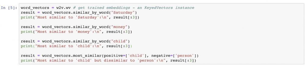
Most similar to 'Saturday':
[('Monday', 0.8932375907897949), ('Sunday', 0.8864969611167908), ('Friday', 0.8746457099914551)]
Most similar to 'money':
[('job', 0.7183666825294495), ('care', 0.7078273892402649), ('advantage', 0.6967247724533081)]
Most similar to 'child':
[('person', 0.8096203804016113), ('artist', 0.7520007491111755), ('woman', 0.742388904094696)]
Most similar to 'child' but dissimilar to 'person':
[('voice', 0.3684268295764923), ('Pamela', 0.3312205374240875), ('smile', 0.33087605237960815)]
Using our embeddings as features in a Neural model
Now that we have our embeddings it’s time to put them into use. We will use them as features for the part-of-speech (POS) tagging model we will develop. A part-of-speech is a grammatical category of a word, such as a noun, verb or an adjective. Given a sequence of words, the task is to label each of them with a suitable POS tag.
We will build a simple neural model for multi-class classification. For now, we will ignore the context of the word we are tagging — our network will take only one word as input and output the probability distribution over all possible POS tags. To train and evaluate our model we will make use of yet another NLTK resource: the data from the CONLL-2000 Shared Task, which has been annotated with POS tags.
Step 1: Preparing the data
Let’s start with importing all necessary libraries and having a look at the CONLL data:
[('Confidence', 'NN'), ('in', 'IN'), ('the', 'DT'), ('pound', 'NN'), ('is', 'VBZ'), ('widely', 'RB'), ('expected', 'VBN'), ('to', 'TO'), ('take', 'VB'), ('another', 'DT')]
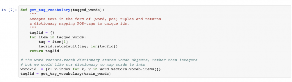
Our first step is to process this data into a model-friendly format — replace all words and tags with their corresponding indexes and split the data into inputs and outputs (tag labels). To do that we will need a dictionary which maps words to their corresponding ids and a similar dictionary for the tags. We will create the latter based on our CONLL training data, but to create the first we will use the vocabulary of our trained embedding model — as it should only contain the words which we are able to represent.
Now it’s time to get our integer, model-friendly data — both for the train and test splits.
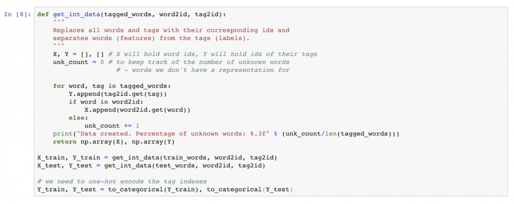
Data created. Percentage of unknown words: 0.143
Data created. Percentage of unknown words: 0.149
So far things seem to be going smoothly, but there is an issue with the get_int_data function. It lies in our handling of the unknown words. If we simply discarded them from the train and test data, as we did just now, we would be running into the risk of fooling ourselves that our model performs better than it does in reality. In addition, our results on the test data would not be comparable to those obtained using a different set of embeddings.
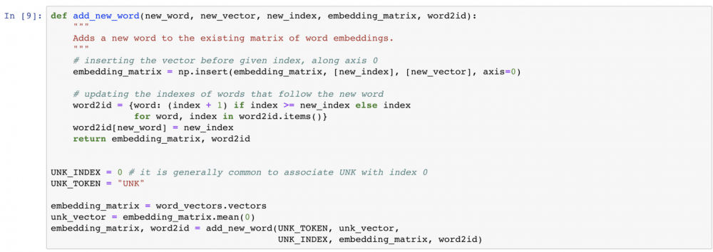
We will fix this problem by adding a new word to our vocabulary — the ‘UNK’, which will represent all words we don’t have an embedding for. But adding this word to the vocabulary means it will need to have a corresponding embedding, not present in our representations. One solution would be to retrain Skip-gram after having replaced some occurrences of low frequency words in our training data with an ‘UNK’ token. But we will approach this problem from a different angle by approximating the UNK’s vector with a mean of all existing embeddings. After doing so, we will add this new representation to the matrix of all other embeddings.
Now that we have created the generic ‘UNK’ word, we will modify the get_int_data function to associate each out-of-vocabulary word with the UNK’s index:
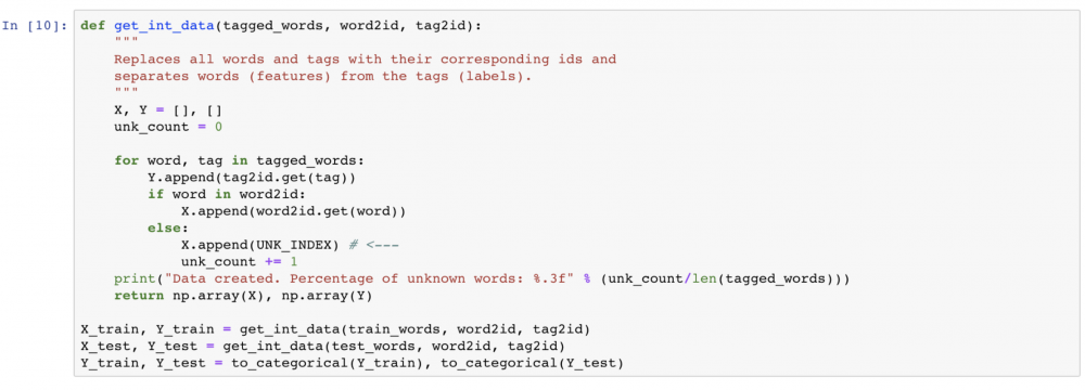
Data created. Percentage of unknown words: 0.143
Data created. Percentage of unknown words: 0.149
Step 2: Defining and training the model
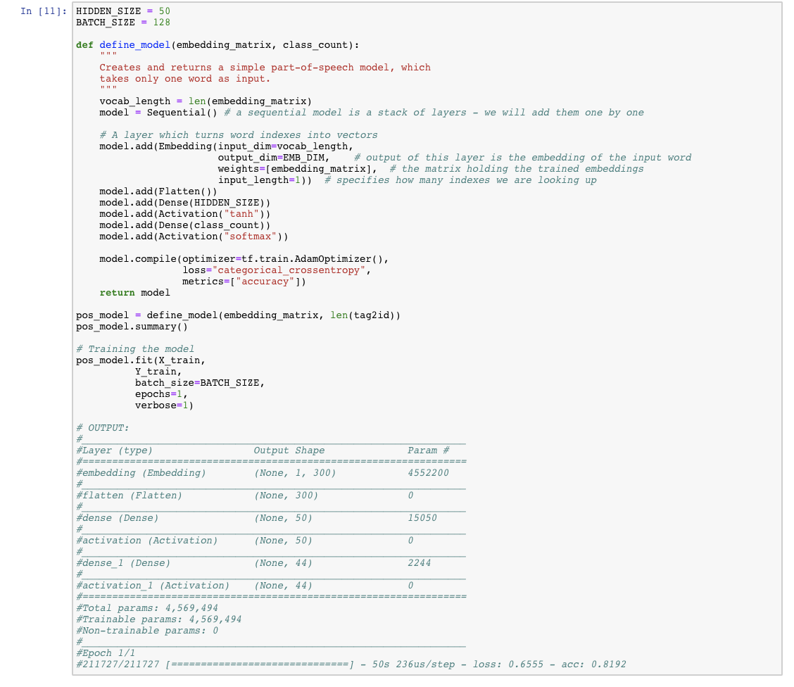
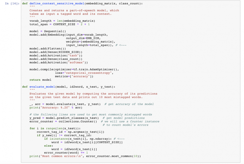
Our next step is to define the model for POS classification. We will do so using TensorFlow’s implementation of the Keras API. Our model will take as input an index into the word embedding matrix, which will be used to look up the appropriate embedding. It will have one hidden layer with the tanh activation function and at the final layer will use the softmax activation — outputting a probability distribution over all possible tags.
Step 3: Evaluating the model
Now that we have a trained model it’s time to see how well it’s performing on the unseen data. We will use it to tag the words from the test data and calculate the accuracy of its predictions: the ratio of the number of correct tags to the number of all words in the test set. To get more insight, we will also determine what are the most commonly mis-tagged words.
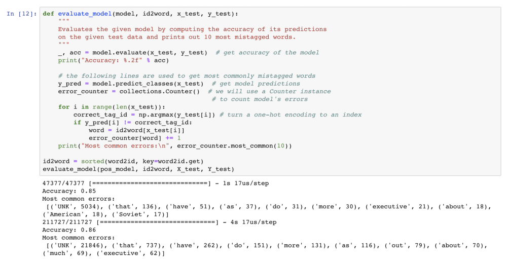
As expected, our model performs the worst when tagging the unknown words. The accuracy is 85%, which is not too bad, but we can do better. Let’s try improving the model by making the classification context-dependent!
Step 4: Building a context-dependent model
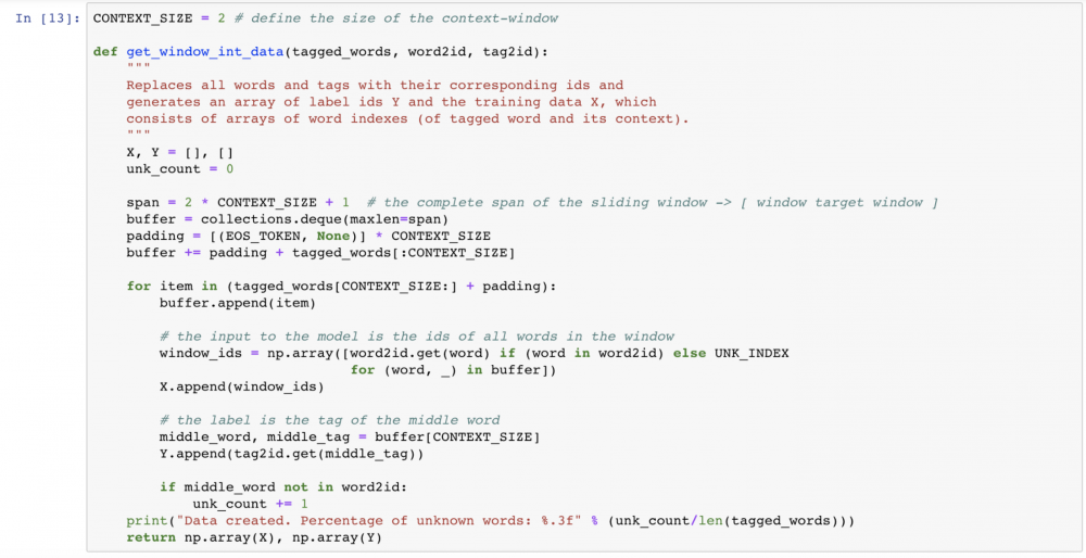
We will now alter the model built in the previous steps to take more than one word index as input. In addition to the index of the classified word we will feed in the indexes of two words to its left side and two words to its right side — all in the order of their appearance in the training data.
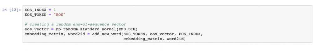
Apart from redefining our model we also need to adjust the way we process the CONLL data: the X_train and X_test will now consist of arrays of indexes, rather than single indexes. We will use a sliding-window approach to retrieve all word spans of length 5 — each consisting of the tagged word and its context-words. For each such span, the corresponding label will be the tag of the middle word. To represent the missing contexts of words at the beginning and the end of the training data sequence we will use a new, special word — the end-of-sequence (EOS). We will add EOS using the previously defined add_new_word function, in a similar way to how we have added UNK:
Now it’s time to prepare the data for our context-dependent model:
Our next step is defining the model. It will be very similar to the simple model from our previous steps. In fact, the only thing that will change is the Embedding layer, which will now take 5 word indexes instead of 1. We will also slightly alter our evaluation function — to support the structure of our new training data.
That’s it! Let’s train and evaluate our new context-dependent model!
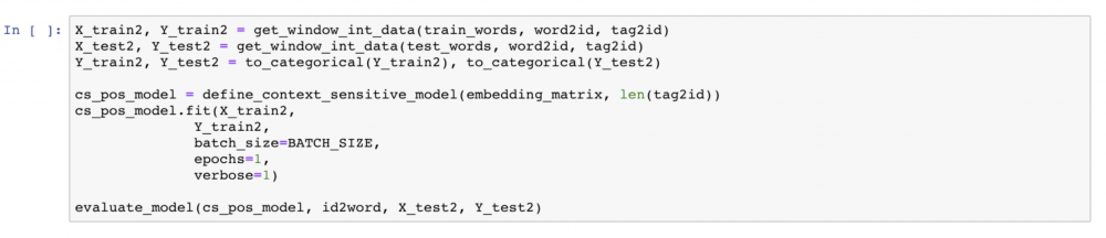
Our accuracy jumped up to 91%! It looks like adding the context really helped with tagging the unknown words and also helped to disambiguate other words. We could probably do even better with stronger embeddings — if you want you can retrain Skip-gram on a bigger corpus and see how the performance of the POS model improves. An easy extension is to train on the Text8 corpus (http://mattmahoney.net/dc/textdata.html) — gensim provides a class specifically designed to iterate over the sentences in Text8 (gensim.models.word2vec.Text8Corpus).
Closing remarks
Throughout this tutorial we have covered:
• How to train our own embeddings using the gensim library
• How to process text data to feed into a neural model
• How to use pre-trained word embeddings in Keras models
• How to build simple context-dependent and context-independent word classification models
Hopefully it has helped you understand word embeddings a bit better and get a feeling for developing models trained on text data. Although in this tutorial we have trained and used our own embeddings, in practice one would often use publicly available vectors which were trained on very large datasets, containing billions of words. One commonly used set of embeddings is the word2vec GoogleNews vectors (https://code.google.com/archive/p/word2vec/) and, conveniently, gensim provides a function to load these vectors (KeyedVectors.load_word2vec_format).
Importantly, not all embeddings are created equal. Meaning is a complex concept and there are multiple axes along which words can be similar. One should be aware that different design decisions and hyperparameter settings often affect the types of similarity reflected in the embeddings. For example, setting Skip-gram’s window to higher values results in capturing similarities that are more topical, domain-related. The way one defines a word’s context also determines what is captured in the embeddings. Defining the contexts as word’s closest neighbours, like in Skip-gram, results in vectors that capture mostly relatedness(e.g. the word cinema would be similar to popcorn). An alternative is to derive contexts from the word’s syntactic dependency relations (subject, object etc.). This leads to capturing semantic similarity which measures the extent to which words share similar functional roles (e.g. cinema would be similar theater). Which embeddings are better will depend on the specific task they are meant to be used for.
Suggested readings
1. To understand Skip-gram
A great introduction to the vector space models of meaning (including Skip-gram)
• Chapter 6 from Daniel Jurafsky and James H Martin. Speech and language processing (3rd ed. draft). https://web.stanford.edu/~jurafsky/slp3/, 2017.
A very good read to delevop understanding of Skip-gram’s objective
• Yoav Goldberg and Omer Levy. word2vec explained: Deriving Mikolov et al.’s negative sampling word-embedding method, 2014.
The original Skip-gram papers
• Tomas Mikolov, Kai Chen, Greg Corrado, and Jeffrey Dean. Efficient estimation of word representations in vector space. ICLR Workshop, 2013.
• Tomas Mikolov, Ilya Sutskever, Kai Chen, Greg S Corrado, and Jeff Dean. Distributed representations of words and phrases and their compositionality. Proceedings of the 26th International Conference on Neural Information Processing Systems, 2013.
2. Additional
For more on capturing different types of similarity and how it can affect the model’s performance:
• Omer Levy and Yoav Goldberg. Dependency-based word embeddings. In Proceedings of the 52nd Annual Meeting of the Association for Computational Linguistics, 2014.
• Douwe Kiela, Felix Hill, and Stephen Clark. Specializing word embeddings for similarity or relatedness. In Proceedings of the 2015 Conference on Empirical Methods in Natural Language Processing, 2015.
On how different hyperparameter settings affect the performance:
• Omer Levy, Yoav Goldberg and Ido Dagan. Improving distributional similarity with lessons learned from word embeddings. Transactions of the Association for Computational Linguistics, 2015.
FastText embeddings: a simple extension of Skip-gram which exploits the subword information. This allows for graceful handling of the unknown words and can lead to improved performance:
• Piotr Bojanowski, Edouard Grave, Armand Joulin, and Tomas Mikolov. Enriching word vectors with subword information. Transactions of the Association for Computational Linguistics, 2017.
3. For more on POS tagging
• Chapter 8 from Daniel Jurafsky and James H Martin. Speech and language processing (3rd ed. draft). https://web.stanford.edu/~jurafsky/slp3/, 2017.
4. References for ELMO and Glove — the embedding models mentioned in the introduction
• Matthew E. Peters, Mark Neumann, Mohit Iyyer, Matt Gardner, Christopher Clark, Kenton Lee, and Luke Zettlemoyer. Deep Contextualized Word Representations. Proceedings of NAACL-HLT, 2018.
• Jeffrey Pennington, Richard Socher, Christopher D. Manning. GloVe: Global Vectors for Word Representation. Proceedings of the 2014 Conference on Empirical Methods in Natural Language Processing, 2014.

About the author
Paula is a Computer Science PhD student at the University of Cambridge. She specialises in Natural Language Processing and her main research interests include cross-lingual learning, low-resource learning and developing models for languages with complex word structures.
Subscribe to Our Newsletter
For more Data Science tutorials, sign up to our bi-weekly newsletter! Contains industry news, interviews, popular resources and latest Cambridge Spark news.
-1.png)
Enquire now
Fill out the following form and we’ll contact you within one business day to discuss and answer any questions you have about the programme. We look forward to speaking with you.
